
As communication systems push into millimeter-wave frequencies and high-speed digital designs approach 10+Gbps data rates, signal degradation becomes the limiting factor in system performance. At these frequencies, a PCB trace is no longer a simple conductor—it's a Transmission Line where every geometry variation, material property, and manufacturing artifact affects Signal Integrity. Insertion Loss and reflection, the two primary degradation mechanisms, determine whether your design performs reliably or fails catastrophically.
Understanding how to minimize these losses separates successful high-frequency designs from expensive prototypes that never meet specifications. This knowledge applies across applications from 5G base stations to Automotive Radar to high-speed data center interconnects.

Before addressing mitigation strategies, it's essential to understand what causes signal degradation in high-frequency PCBs.
Insertion Loss represents the reduction in signal power as it travels through a transmission path. It's expressed in decibels (dB) and includes all losses between the input and output of the Transmission Line:
Total Insertion Loss = Conductor Losses + Dielectric Losses + Radiation Losses + Leakage Losses
Conductor losses arise from the finite conductivity of copper. At DC, this is simply I²R resistance. At high frequencies, Skin Effect forces current to flow in an increasingly thin layer near the conductor surface, dramatically increasing effective resistance. A 1mm wide trace at 1 GHz uses only about 21% of its cross-sectional area, effectively reducing width to approximately 0.21mm.
Dielectric losses occur as the alternating electric field in the transmission line causes molecular polarization in the substrate material. Energy dissipates as heat. Dielectric loss is characterized by the loss tangent (tan δ)—lower values indicate better performance. Standard Fr-4 has tan δ around 0.02 at GHz frequencies, while high-performance Rf Materials have tan δ below 0.005.
Radiation losses occur when the transmission line radiates energy. Microstrip traces radiate more than stripline, and radiation increases with frequency. Poor Grounding and discontinuities amplify radiation losses.
Leakage losses through the dielectric are typically negligible at PCB frequencies but can matter at very high frequencies or for specialized materials.
Reflection occurs when a signal encounters impedance discontinuities along its path. The reflection coefficient (Γ) quantifies this:
Γ = (ZL - Z0) / (ZL + Z0)
Where ZL is the load impedance and Z0 is the Characteristic Impedance of the transmission line. When ZL equals Z0, reflection is zero. Any mismatch causes reflections that travel back toward the source, distorting the signal waveform.
Sources of reflection include:
Material choice fundamentally determines high-frequency performance. Making informed material selections early prevents problems that cannot be fixed during layout.
The Dielectric Constant affects impedance, wavelength, and coupling between traces. Key considerations:
Loss tangent directly determines dielectric loss at your operating frequency. Higher frequencies increase loss exponentially, making low-Df materials essential above 10 GHz:
Rogers Ro4003c: Hydrocarbon ceramic filled, Dk 3.38, Df 0.0027 at 10 GHz. Excellent balance of electrical and mechanical properties. Lower cost than pure Ptfe materials. Widely used for RF and microwave applications up to 20 GHz.
Rogers RT/duroid 5880: Ptfe fiberglass, Dk 2.2, Df 0.0009 at 10 GHz. Exceptional loss performance but mechanically softer and more expensive. Preferred for applications below 77 GHz requiring minimum loss.
Isola I-Speed: Modified FR-4 with improved loss characteristics, Df ~0.006. Compatible with standard PCB processing, lower cost than Rogers materials. Good choice for applications to 15 GHz.
Megtron 6/7: Low-loss epoxy, Df ~0.002. Designed for high-speed digital applications, also suitable for RF. Compatible with standard processing.
Some materials have processing constraints:
Trace geometry directly determines impedance and loss. Optimizing geometry is one of the most effective ways to improve high-frequency performance.
Microstrip: Trace on outer layer with Ground Plane beneath. Simple to manufacture but higher radiation losses and sensitivity to surface contamination. Suitable for frequencies to approximately 30 GHz with careful design.
Stripline: Trace between two ground planes. Lower radiation losses and better Shielding. More complex manufacturing but provides consistent impedance and reduced sensitivity to surface effects. Preferred for very high frequencies or applications requiring minimal Emi.
Grounded Coplanar Waveguide (Gcpw): Trace with ground planes on either side and below, all connected with vias. Combines benefits of microstrip and stripline. Excellent for mm-wave frequencies. The side grounds improve mechanical robustness and reduce radiation.
For a given impedance target, trace width and dielectric thickness trade off:
For very high frequencies (above 20 GHz), consider ounce copper weights above standard 1oz. Heavier copper reduces Skin Effect resistance, but requires adjusted geometries for Impedance Control.
Manufacturing tolerances affect impedance accuracy. For high-frequency designs:
Vias introduce discontinuities that cause reflection and increase loss. Careful via design minimizes these effects.
A via has parasitic inductance and capacitance that create resonance effects:
Minimize via discontinuities through design:
Back-drilling removes the unused portion of through-hole vias, eliminating stub effects. For very high frequencies (above 20 GHz):
Ground vias adjacent to signal vias provide return paths:
High-speed serial interfaces (56G/112G PAM4, PCIe 5/6, etc.) demand careful differential pair design to minimize skew and mode conversion.
Coupling coefficient affects differential impedance:
Skew—difference in propagation delay between pair members—causes mode conversion from differential to common-mode signals:
For differential pairs transitioning layers:
Every transition between different transmission structures creates discontinuity. Managing transitions carefully is essential for overall performance.
Connector footprints often create impedance discontinuities:
Component mounting pads create capacitance that lowers impedance at the pad:
For board-edge launches to coaxial connectors:
At high frequencies, the power distribution network (PDN) affects Signal Integrity through multiple mechanisms.
Currents drawn by active components flow through the PDN. If PDN impedance is high, switching noise couples into signals:
When multiple outputs switch simultaneously, PDN voltage droop can affect signal levels:
High-frequency design requires verification beyond DC continuity testing.
For designs above 10 GHz, 3D Electromagnetic Simulation is essential:
Simulation accuracy depends on material model accuracy. Work with your material supplier for dielectric properties at your operating frequency.
Tdr measurements reveal impedance discontinuities:
Vna measurements characterize full transmission performance:
Communicate impedance requirements clearly to your manufacturer:
Surface finish affects high-frequency loss and bonding:
Solder mask affects microstrip trace impedance:
Design to a total loss budget, allocating allowable loss to each segment:
Minimizing insertion loss and reflection in high-frequency PCBs requires attention to every design detail. From material selection through trace geometry, via design, and manufacturing communication, each decision affects final performance.
The key principles are straightforward: choose materials with appropriate loss characteristics, maintain consistent impedance through careful geometry control, minimize discontinuities from vias and transitions, and verify designs through simulation and measurement. But applying these principles requires expertise developed through experience and collaboration with materials suppliers, manufacturers, and measurement specialists.
As frequencies continue rising—toward 5G Millimeter Wave bands, Automotive Radar, and 200+Gbps data links—the techniques for loss minimization become even more critical. Designs that worked at 10 GHz fail at 30 GHz without careful attention to the principles outlined here. Investing in high-frequency expertise and simulation capabilities enables successful designs that meet performance requirements on the first spin.
Work closely with your Pcb Manufacturer throughout the design process. Their expertise in material handling, Controlled Impedance processing, and high-frequency fabrication complements your design capabilities. Early collaboration prevents costly redesigns and ensures that designed-for performance becomes manufactured reality.
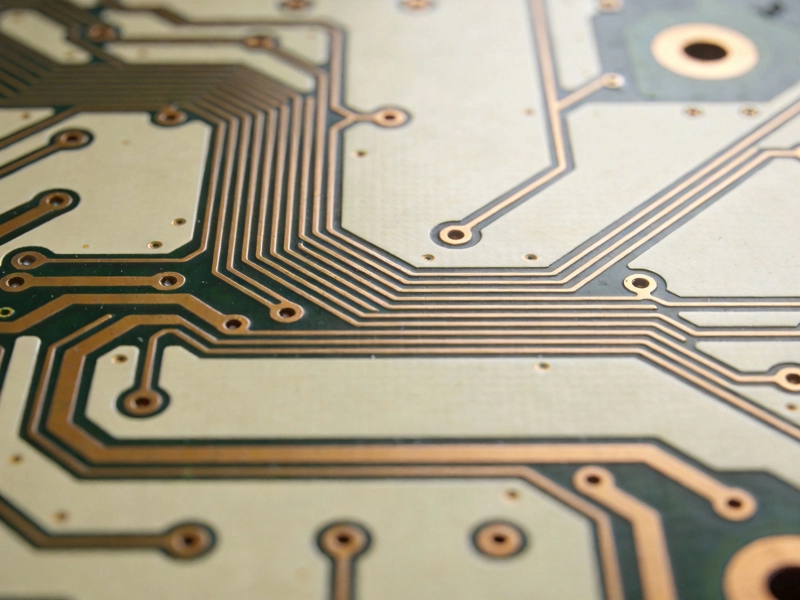
Demystifying Impedance Control: Core High Frequency PCB KnowledgeJuly/09/2026
High Frequency PCB Knowledge: Best Practices for Grounding and ShieldingOctober/12/2026

High Frequency PCB Knowledge: The Difference Between High-Speed and High-FrequencySeptember/17/2026
Key High Frequency PCB Knowledge for Successful RF Circuit DesignSeptember/07/2026
Advanced High Frequency PCB Knowledge: Using Simulation Tools for Better ResultsSeptember/29/2026
Essential High Frequency PCB Knowledge for Hardware Engineers and DesignersJune/15/2026
High Frequency PCB Knowledge: Managing Crosstalk and EMI in Dense LayoutsAugust/11/2026
The Engineer's Guide to High Frequency PCB Knowledge and Stack-up DesignJuly/31/2026