Open Nav

Ask any engineer who has designed a high-speed digital board or an RF frontend, and they will tell you the same thing: getting Impedance Control right is one of those topics that looks deceptively simple on the surface and reveals hidden complexity the moment you try to implement it in a real stack-up. The concept of Characteristic Impedance—a property of a Transmission Line that determines how voltage and current waves propagate along a conductor—is straightforward. The practice of controlling that impedance within tight tolerances across a multilayer PCB fabricated by an external manufacturer, assembled with solder paste, and deployed in a variable thermal environment, is anything but.
Yet Impedance Control is non-negotiable for any PCB operating above approximately 500 megahertz or carrying high-speed digital signals with rise times faster than a few nanoseconds. At these frequencies, the wavelength of the signal approaches the physical dimensions of the traces on the board, and the way the PCB routing interacts with the electromagnetic field becomes the dominant factor in Signal Integrity. A mismatched impedance causes Signal Reflection, ringing, and data corruption that no amount of firmware optimization can fix. This article cuts through the jargon and gives you the foundational knowledge you need to design, specify, and source Controlled Impedance PCBs with confidence.
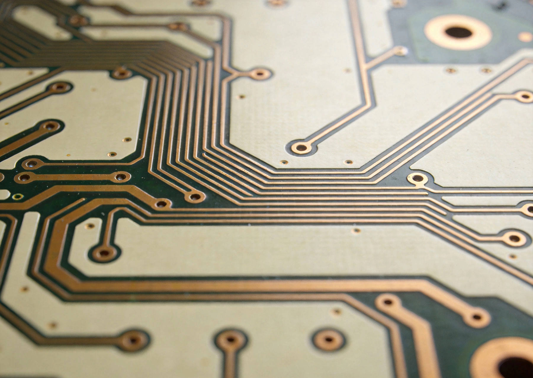
Electrical impedance is the opposition that a circuit presents to alternating current, measured in ohms. In DC circuits, resistance is the only parameter that matters. At high frequencies, the behavior of conductors and dielectrics changes in ways that introduce additional components of opposition: inductive reactance from the magnetic field around the current-carrying trace, and capacitive reactance from the electric field between the trace and the reference plane below it. The combination of resistance, inductance, and capacitance at a given frequency determines the total impedance.
On a PCB trace that is part of a Transmission Line, the Characteristic Impedance—often denoted as Z0—is the impedance that a high-frequency signal sees as it travels along the trace, assuming the trace is infinitely long and terminated with exactly that impedance. When the actual impedance of the trace differs from the impedance of the driver and receiver at each end, a portion of the signal reflects back toward the source. At the board level, these reflections cause the signal waveform to distort, creating overshoot, undershoot, and ringing that degrades signal quality and can cause false triggering in digital circuits or power amplifier instability in RF designs.
The magnitude of the reflection is determined by the impedance mismatch coefficient, sometimes called the reflection coefficient. A 10 percent impedance mismatch on a 50-ohm line produces a reflection of about 5 percent of the signal amplitude. A 20 percent mismatch produces a reflection of roughly 10 percent. For sensitive high-speed serial data links operating at gigabit per second rates, even a 5 percent mismatch can push bit error rates above acceptable limits.
Understanding transmission line theory is essential for anyone working with Controlled Impedance PCBs. The good news is that you do not need a graduate degree in electromagnetic theory to design reliable controlled impedance boards—you need to understand a few key concepts and how they map to practical PCB design decisions.
PCB traces carrying high-frequency signals are designed as transmission lines, and the geometry of the trace relative to its surrounding materials determines its characteristic impedance. The two most common transmission line geometries on PCBs are microstrip and stripline.
A microstrip trace runs on the surface of the board, with a reference plane (typically a ground plane or power plane) on the layer immediately below it. The electromagnetic field that surrounds the signal trace extends partly into the air above the board and partly into the dielectric material below. This dual-dielectric environment makes microstrip impedance slightly dependent on the thickness and Dielectric Constant of the air above the trace, which varies with component height and surrounding geometry. Microstrip is the simpler geometry to manufacture and is the preferred choice for most RF applications up to approximately 30 gigahertz.
A stripline trace is embedded between two reference planes, fully surrounded by dielectric material. The electromagnetic field is contained entirely within the board, which makes stripline impedance more predictable and less sensitive to external geometry changes. Stripline also provides better shielding from external interference and from crosstalk with adjacent traces, which makes it preferable for very high-speed digital applications and multilayer high-density designs where signal isolation is critical. The trade-off is that stripline is more complex to manufacture because the trace must be routed between internal planes, and via stubs can create resonance problems that require back-drilling to eliminate.
For a given trace geometry, four parameters determine the characteristic impedance: trace width, trace thickness, the distance between the trace and its reference plane (the dielectric thickness), and the Dielectric Constant of the material between them. Understanding how each parameter affects impedance helps you adjust your stack-up to hit your target value.
Increasing trace width increases the capacitance between the trace and the reference plane, which decreases impedance. This is the most commonly adjusted parameter because trace width can be changed in the layout without altering the board's physical construction. For a standard Fr-4 board with 1.6-millimeter thickness and 1-ounce copper, the trace width needed for 50 ohms on a surface microstrip is approximately 2.9 millimeters—surprisingly wide for a board with fine-pitch components. This is why controlled impedance traces often need to be routed on dedicated layers with wider trace geometries rather than squeezed into the same routing channels as the board's digital signals.
Increasing the distance between the trace and the reference plane reduces the capacitance between them, which increases impedance. This is a powerful lever for adjusting impedance, but it requires changing the PCB stack-up—moving the reference plane further from the signal layer. This affects all traces on that layer and has implications for board thickness and layer count.
Increasing trace thickness has a smaller effect than width or dielectric thickness, but it does increase impedance slightly by reducing resistance and slightly changing the field distribution around the trace. In practice, trace thickness is determined by the copper weight specification (0.5 oz, 1 oz, 2 oz), and the designer works within those constraints.
The dielectric constant of the material directly affects impedance. A lower dielectric constant produces a higher impedance for the same geometry. Standard Fr-4 has a dielectric constant of approximately 4.2 to 4.5 at 1 megahertz, but this value changes with frequency—it drops to around 4.0 at 1 gigahertz and continues decreasing at higher frequencies. For precise impedance control, you need to use the dielectric constant value at your actual operating frequency, not the datasheet value measured at low frequency. High-frequency Pcb Materials like Rogers RO4003C have more stable and lower dielectric constants (3.38 for RO4003C) that do not vary as much with frequency, which makes them preferable for applications above approximately 5 gigahertz.
The PCB stack-up is the arrangement of copper layers, prepreg cores, and Dielectric Materials that make up the finished board. For controlled impedance designs, the stack-up is not an afterthought—it is the primary design artifact that determines whether your impedance targets are achievable.
Each high-speed signal layer in your stack-up needs an adjacent reference plane. This reference plane serves as the return path for the signal current and establishes the transmission line geometry. The reference plane should be a solid copper pour connected to ground in almost all cases. A power plane can serve as a reference plane, but it introduces complications because power planes can have voltage transients and noise that affect signal quality. Ground planes are preferred because they provide a stable, low-impedance return path that minimizes ground bounce and crosstalk.
For multilayer boards, the most reliable stack-up for impedance control places each signal layer directly adjacent to a ground plane on the layer immediately below it. This creates a consistent reference geometry that is straightforward to model and manufacture. Routing signals across layers that do not have an adjacent ground plane—such as a signal layer between two signal layers—makes impedance control significantly more difficult because the return path must find an indirect route to ground.
Many high-speed signals, including USB, PCIe, HDMI, and Ethernet, are transmitted as differential pairs—two traces carrying equal and opposite signals. The impedance specification for differential pairs is called differential impedance, and it is different from the single-ended impedance of each trace. Differential impedance is approximately twice the single-ended impedance when the traces are spaced far apart, but it drops as the traces are routed closer together because of the coupling between them. For a 50-ohm single-ended system, the differential impedance target is typically 100 ohms, though this varies by application.
Designing differential pairs for controlled impedance requires managing both the single-ended impedance of each trace and the coupling between them. The key geometry parameters are trace width, trace spacing, and the distance to the reference plane below. Tight, consistent coupling between the pair traces is important because it determines how much of the signal energy is carried in differential mode versus common mode. Uncoupled or loosely coupled differential pairs are more susceptible to common-mode noise and electromagnetic interference. Most impedance calculation tools can compute both single-ended and differential impedance simultaneously, and it is good practice to use these tools rather than estimating geometries manually.
No manufacturing process produces PCBs with perfectly uniform dimensions, and impedance tolerance is a measure of how much variation from the target value is acceptable. Typical tolerances for controlled impedance PCBs are plus or minus 10 percent for standard commercial applications, plus or minus 7 to 8 percent for telecommunications and networking equipment, and plus or minus 5 percent or tighter for aerospace, military, and high-speed serial applications.
Tighter tolerances are more expensive to achieve because they require more precise control over dielectric thickness, trace width, and copper plating uniformity. They also require more careful characterization and verification through impedance test coupons measured with Time Domain Reflectometry on every panel. When specifying impedance tolerances, match the requirement to the actual application need. Specifying plus or minus 5 percent tolerance when plus or minus 10 percent would suffice increases cost and can unnecessarily constrain manufacturing options.
Designing a controlled impedance PCB starts with calculation: determining what trace geometry is needed to achieve the target impedance on your chosen stack-up. For most practical designs, engineers use field-solver software or impedance calculators rather than analytical formulas, because the field distribution around a real trace in a real PCB is too complex for simple equations to model accurately.
Analytical equations like the IPC-2141 formulas for microstrip and stripline impedance provide reasonable estimates for simple geometries at lower frequencies, but they break down for non-standard stack-ups, tightly coupled differential pairs, and frequencies above a few gigahertz. Modern PCB design tools include 2D field solvers that solve Maxwell's equations numerically for the specific geometry of your trace, reference plane, and Dielectric Materials. These tools are significantly more accurate than empirical equations and are the standard for serious impedance-controlled designs.
When working with your Pcb Manufacturer, share your impedance calculation parameters including the dielectric constant value you used, the target impedance, the tolerance, and the specific geometry (trace width, spacing, copper weight, and dielectric thickness). A quality manufacturer will model the stack-up using their own field solver, verify that the calculations match, and build impedance test coupons that are measured and reported with every production panel. If the manufacturer is using different dielectric constant values or stack-up dimensions than your calculations assumed, they should flag the discrepancy and propose a correction before production begins.
The trace width required to achieve 50 ohms on a standard microstrip stack-up is often wider than you might expect. On a typical 1.6-millimeter board with 1-ounce copper and standard FR-4, the 50-ohm microstrip trace width is approximately 2.8 to 3.1 millimeters, depending on the exact dielectric constant and prepreg compression during lamination. This is much wider than the 0.1 to 0.2 millimeter traces used for dense digital routing on the same board. For this reason, controlled impedance traces typically require dedicated routing channels and cannot simply be squeezed into the same routing area as other signals.
Planning for controlled impedance routing should begin at the earliest stages of stack-up design. Identify the number of controlled impedance signal layers you need, whether they are single-ended or differential, what impedance values are required, and what routing density you need on each layer. This information determines the minimum board thickness, the minimum layer count, and the minimum trace geometry requirements. Sharing this plan with your Pcb Manufacturer early allows them to optimize the stack-up for both impedance control and overall board cost.
Design calculations are only half the challenge. The manufacturing process introduces variations that can shift the finished impedance away from the calculated target, and managing these variations is what separates a reliable controlled impedance design from one that fails inspection.
The thickness of the dielectric material between the trace and its reference plane does not stay exactly constant across a production panel. Prepreg—the partially cured fiberglass sheets that bond layers together during lamination—compresses under heat and pressure, and the amount of compression varies with temperature, pressure, and the specific resin content of the prepreg. This compression reduces the dielectric thickness from its pre-lamination value, which increases capacitance and decreases impedance. Manufacturers control this by using calibrated prepreg materials, maintaining precise lamination pressure profiles, and measuring actual dielectric thickness on production panels using cross-section coupons.
After plating, the copper on the outer layers is not exactly the thickness specified by the copper weight. The plating process adds copper unevenly, with more copper depositing on the surface than on the sidewalls of the traces, which affects the trace geometry. Additionally, the etching process that defines the trace shapes removes copper from the sides of the traces as well as the top, making the finished trace slightly narrower than the artwork dimensions. This is called etch factor, and it is compensated for in the artwork by making the traces slightly wider than the final target width. Manufacturers develop etch compensation factors based on their specific process parameters, and these factors should be incorporated into the artwork generation for controlled impedance layers.
Surface finishes like ENIG (Electroless Nickel Immersion Gold) or HASL (Hot Air Solder Leveling) add thin layers of metal over the copper traces. While these layers are thin—a few microinches of gold or a few mils of solder—they do affect the effective conductivity and geometry of the trace at very high frequencies. For most applications below 10 gigahertz, the effect is negligible. For microwave applications above 20 gigahertz, the choice of surface finish can measurably affect impedance, and some designers specify specific finishes to manage this effect. Discuss any tight impedance requirements above 15 gigahertz with your manufacturer to determine whether surface finish selection requires special attention.
A well-calculated stack-up can be compromised by routing practices that introduce impedance discontinuities. Even a board with perfectly controlled 50-ohm traces will exhibit Signal Integrity problems if the routing geometry changes abruptly along the signal path.
Via stubs—the unused portion of a through-hole via below the signal layer—create a resonance at frequencies determined by the stub length. A 1-millimeter stub resonates at approximately 37.5 gigahertz (calculated as 75 nanoseconds per inch divided by 2 for the round-trip propagation). For signals operating below this frequency, the stub acts as a capacitive discontinuity that degrades impedance and creates reflections. The standard solution is back-drilling, where the unused portion of the via barrel is mechanically drilled out after plating to remove the stub. Back-drilling is essentially mandatory for high-speed serial links operating above 5 gigabits per second on through-hole via structures.
Reference plane changes—where a signal trace crosses a gap or split in the reference plane—interrupt the return current path and force it to find an alternate route around the discontinuity. This increases loop inductance and creates an impedance discontinuity that can cause reflections and crosstalk. When signals must cross a plane split, stitching vias placed on each side of the signal trace within a few millimeters of the crossing point can provide an alternate return path and minimize the discontinuity. Routing sensitive signals over solid, uninterrupted reference planes is the best practice and should be planned from the beginning of the layout.
Unequal differential pair length introduces skew, where one signal in the pair arrives before the other. At high data rates, skew causes the differential signal to momentarily collapse, creating bit errors. Maintaining pair length matching within approximately 5 mils (0.127 millimeters) per gigabit per second of data rate is a good rule of thumb, though more stringent matching may be required for specific protocols. Meander routing to compensate for length differences should be applied symmetrically in the coupled region and ideally in an uncoupled section outside the main routing channel.
Manufacturing a controlled impedance PCB without testing it is like designing a structural beam without checking its load rating. Verification is essential to confirm that the process delivered what was specified.
Every controlled impedance PCB production panel should include impedance test coupons—short trace segments built into the panel frame under the same conditions as the production traces. These coupons are measured using Time Domain Reflectometry, which sends a fast pulse down the trace and analyzes the reflected waveform to calculate impedance. Tdr provides direct, quantitative verification of the impedance on each controlled impedance layer and each trace type (single-ended and differential). The measurement should be taken at multiple locations across the panel to verify uniformity.
When commissioning a new stack-up or qualifying a new manufacturer, request a full impedance test report for the first production panels. This report should include the measured impedance on each coupon, the deviation from target, the panel uniformity data, and any corrective actions taken if measurements fell outside tolerance.
Beyond impedance characterization, every controlled impedance board should receive standard electrical continuity and isolation testing. Continuity testing verifies that all traces and nets are electrically connected. Isolation testing verifies that adjacent nets are not shorted and that there is adequate resistance between isolated circuits. These tests catch manufacturing defects like trace opens, shorts, and contamination that could compromise signal integrity even if the impedance itself is correct.
Single-ended impedance is the impedance of a single trace measured relative to its reference plane. It is the fundamental impedance parameter for any transmission line. Differential impedance is the impedance of a pair of traces carrying equal and opposite signals, measured between the two traces. For a well-coupled differential pair, the differential impedance is approximately twice the single-ended impedance of each trace. Common differential impedance targets include 90 ohms (used by USB 3.0 and PCIe), 100 ohms (used by Ethernet and USB 3.1), and 85 ohms (used by HDMI and DisplayPort).
FR-4 can be used for applications up to approximately 10 gigahertz, but with certain limitations. FR-4 has higher dielectric loss than specialty high-frequency materials, which increases signal attenuation at very high frequencies. The dielectric constant of FR-4 also varies more with frequency and temperature than specialty materials, which makes impedance prediction less precise. For applications above approximately 5 gigahertz, Rogers high-frequency laminates or similar materials are preferred because they offer lower loss, more stable dielectric constant, and tighter impedance control. Below 5 gigahertz, FR-4 is often acceptable if the board is designed with adequate margins and the manufacturer has experience with controlled impedance on standard materials.
For most high-speed digital applications operating at gigabit per second data rates, an impedance tolerance of plus or minus 10 percent is adequate. For more sensitive applications such as PCIe Gen 4 or 5, 10Gb Ethernet, or SATA interfaces, plus or minus 7 to 8 percent is recommended. For the most demanding high-speed serial links operating above 25 gigabits per second, plus or minus 5 percent or tighter may be necessary to maintain acceptable bit error rates. Always consult the specific protocol specification for the application to determine the actual impedance tolerance requirement.
PCB impedance has a temperature coefficient of approximately plus 50 to 100 parts per million per degree Celsius for standard FR-4. This means that as the board temperature increases, the impedance rises and the dielectric constant changes. For most applications, this variation is small enough to ignore. However, for applications where the board operates over a wide temperature range—such as automotive under-hood electronics or outdoor RF equipment—the temperature drift in impedance may need to be factored into the design margin. Specialty high-frequency materials like Rogers Laminates have lower temperature coefficients, which makes them preferable for temperature-critical applications.
No. Only signals that operate at frequencies where the wavelength is comparable to the trace length require controlled impedance. As a practical guideline, signals with rise times below approximately 1 nanosecond, or frequencies above 500 megahertz, benefit from controlled impedance routing. Slower signals, power and ground traces, and control signals that do not carry high-frequency content can be routed normally without impedance control. Over-specifying controlled impedance for every trace on a board increases cost and routing complexity without providing meaningful benefit.
Controlled impedance PCB design is a discipline that sits at the intersection of electromagnetic theory, materials science, and manufacturing process control. While the underlying physics can fill textbooks, the practical knowledge needed to design and source reliable controlled impedance PCBs is accessible to every engineer willing to invest a modest amount of time in understanding the fundamentals. The key concepts—transmission line geometry, the relationship between trace width and impedance, the role of the reference plane, and the impact of manufacturing variations—form a framework that scales from simple single-ended 50-ohm designs to complex multi-gigabit differential pair routing.
The most successful controlled impedance designs are those where the designer and the manufacturer work as partners from the beginning. Sharing your impedance targets, stack-up preferences, and routing constraints early in the process gives the manufacturer the information they need to optimize the build. Running impedance calculations with the manufacturer's actual dielectric constants and stack-up dimensions, rather than textbook values, eliminates surprises. And verifying the finished boards with Tdr test coupons on every panel ensures that what was designed is what was delivered.
As signal speeds continue to increase and applications push into higher frequency ranges, the importance of controlled impedance design will only grow. Building the knowledge and design habits to handle impedance control confidently today is an investment that pays dividends on every high-speed project you tackle tomorrow.
This article is provided for general informational purposes regarding controlled impedance PCB design fundamentals. Specific design requirements and manufacturing tolerances should be determined in consultation with your PCB manufacturer and based on the electrical requirements of your target application.
The Engineer's Guide to High Frequency PCB Knowledge and Stack-up DesignJuly/31/2026

High Frequency PCB Knowledge: Managing Crosstalk and EMI in Dense LayoutsAugust/11/2026

High Frequency PCB Knowledge: How to Minimize Insertion Loss and ReflectionJuly/21/2026
Essential High Frequency PCB Knowledge for Hardware Engineers and DesignersMay/29/2026

Essential High Frequency PCB Knowledge for Hardware Engineers and DesignersJune/15/2026
Handling Sensitive ComponentsMay/29/2026

Advanced High Frequency PCB Fabrication Techniques for Low Loss PerformanceMay/29/2026

How to Source Reliable Industrial SMT PCB Assembly from Trusted China ManufacturersJuly/29/2026